3 What is machine learning?

It’s hard to come up with a precise definition for machine learning. Broadly, it is a field in the intersection of computer science, statistics, and optimization whose goal is to develop algorithms for data analysis and automated or augmented decision-making. A narrow definition includes problems like supervised learning and unsupervised learning, which we briefly discuss below, but other problems such as reinforcement learning also fall within its scope. Over the past years, many fruitful collaborations between machine learning practitioners and experts in other areas have led to machine learning algorithms applied in various contexts, such as health sciences, natural language processing and so many others. For more reviews about machine learning in economics in particular, see also: Varian (2014), Athey (2017), Mullainathan & Spiess (2017), Athey & Imbens (2017).

One theme we’d like to emphasize throughout this report is that machine learning methods sometimes need to be extended or adapted for particular goals. Shortly we’ll introduce a few key concepts related to machine learning methods, but we’ll do so with an eye towards understanding how and why these methods need to be modified when the goal is causal inference.

3.1 Supervised learning

In supervised machine learning, we have a set of input variables or “covariates” (X) as well as output variables (Y). Given observations of both (X) and (Y), we train an algorithm to find a strategy, or function Y=f(X) that accurately predicts the outcome of interest (Y) in a given data sample. The learning process continues until the algorithm has found a strategy (function) for consistently determining accurate answers. Ultimately, the goal is for the algorithm to be able to predict (Y) “out of sample,” given observations (X) that it has never seen before.

Supervised learning is often equated to the process of a math teacher training a student: the teacher gives the student a database of questions together with the answers (the “training set”), and the student tries to learn strategies to replicate the answers. The teacher further has a set of practice tests and answers (the “validation set”) that the student can use to evaluate which of her strategies works best on questions she hasn’t seen before. The ultimate goal is that when the student gets the final exam with questions she hasn’t seen before (“the test set”), she will perform well compared to other students.

Supervised machine learning is divided into two types of problems: classification and regression. In a classification problem, the outcome variable (Y) is categorical (e.g. “disease” or “no disease”), whereas in a regression problem the outcome variable is a continuous measure (e.g. “length of hospital stay”). An example of classification is the problem of predicting whether a patient has a disease (Y=1) or not (Y=0) given measures of their health status (X). An example of regression is the problem of predicting the length of stay (Y) for a hospital patient given several measures of their health status (X).

In practice, supervised learning works by fitting a predictive model – a function f whose input is a vector of covariates (X) and whose output is a guess for the value of the outcome. In Figure 3.1, the function f is a regression tree, where the tree “splits” the data according to values of covariates, and the model predicts the value of the outcome using the sample mean of observations in the “leaves” or final nodes of the tree.

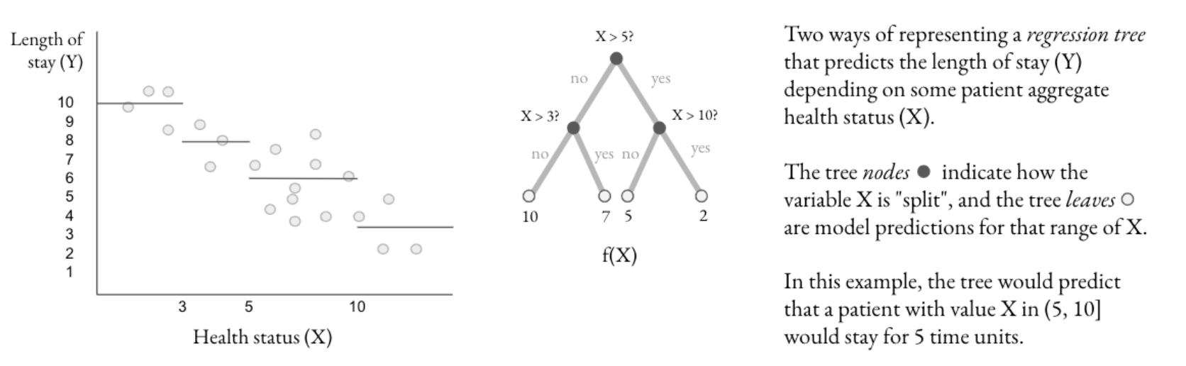
Figure 3.1: A regression tree.

The process of finding such a model usually involves the minimization of some mathematical criterion that measures the prediction error. For example, in a regression problem, given a data set consisting of pairs (X, Y) and a set of possible models (as shown in Figure 3.2, e.g regression trees of different depth), we might select the function for which the mean squared error between observed and predicted outcomes is small. Continuing the regression example we mentioned above: we would like to select a function f such that the length of hospital stay it predicts, f(X), is close to the length of stay we actually observed in the data Y in terms of their average squared difference.

Moreover, in most cases, we want this model to be useful beyond the dataset that was used to find the function. That is, we would like the model to perform well at predicting the outcome Y for a value of X that it has not seen before. This is often accomplished by separating the dataset into three subsets, as illustrated in Figure 3.2: the “training” dataset, which is used to fit different predictive models of increasing complexity, the “validation” set used to select among them, and the “test” dataset in which the functions are evaluated.

Continuing the example above, we might use the training dataset to fit regression trees of different depths. Deeper trees will necessarily be better at estimating the value of the outcome on the training dataset. However, if they find patterns in the training dataset that are not present in unseen observations, they will not be able to produce good predictions for those unseen observations – in machine learning jargon, we say that there is overfitting. Indeed, in the case of a regression tree, it is possible to perfectly fit the data by splitting the data into smaller and smaller leaves until only one observation per leaf remains; although it will fit perfectly in the training data, since the mean value of observations in the leaf is equal to the value of the outcome for the single observation in that leaf, such a deep tree will not do very well predicting outcomes for new datasets. In order to avoid that, we observe the performance of each decision tree at predicting outcomes in the “validation” dataset, and select the best one. The performance of the selected model is then assessed on the “test” set.

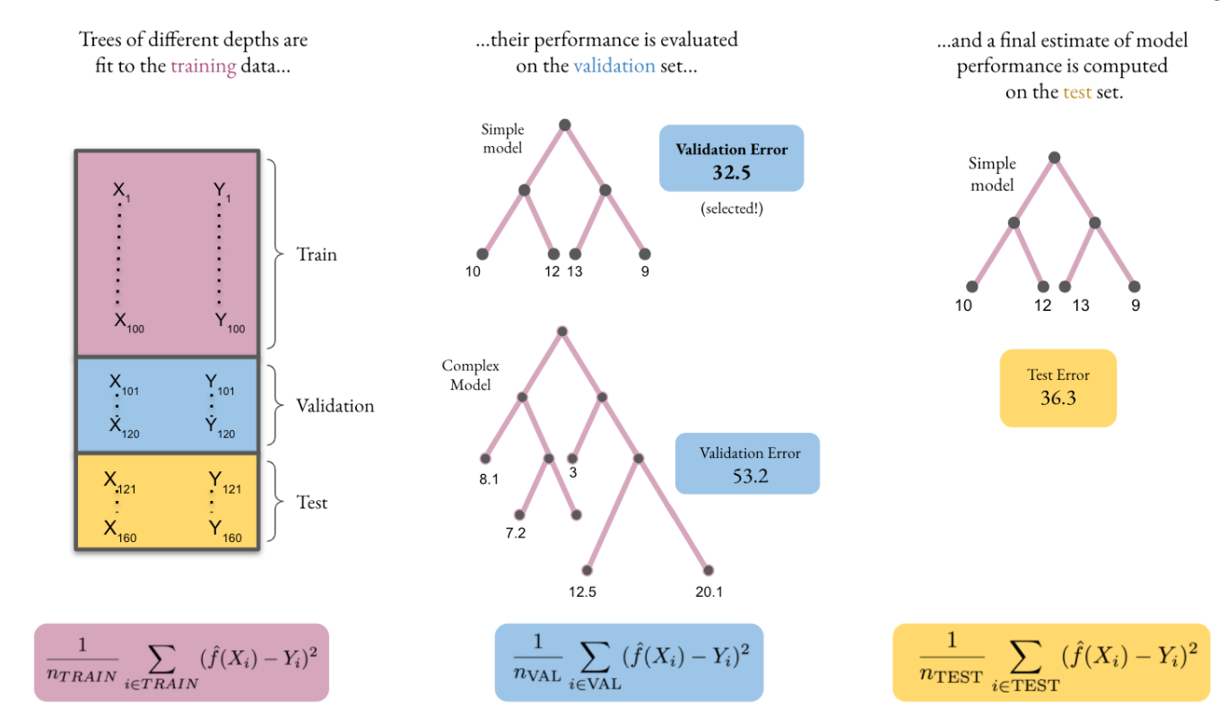
Figure 3.2: Train, test, split..

In practice, often the training and validation data are combined and the validation step is repeated multiple times across different folds of the data, in a practice referred to as cross-validation. More precisely, the training data is split into, say, five folds. For each of the five folds, 20% of the training data in the fold is used for validation, while the remaining 80% of the training data is used to estimate a set of models, for example ranging from simple to complex. The performance of each of the models is assessed using the validation fold. After repeating the exercise for all five folds, the researcher selects the model complexity that performed the best averaged across all five validation exercises. Finally, a model with that selected level of complexity is estimated using the entire training dataset, and this is the final model used to make predictions.

Supervised learning vs causal inference

It is important to emphasize that the goal of predicting an outcome contrasts to a more traditional social science objective of estimating how different factors affect the outcome. Since in supervised learning the goal is just to get the right answer, i.e., find a predictive model such that f(x) = y, it is not necessary to inspect the model or even understand how it works in order to assess whether it performs well in test set predictions. This is different from how behavioral scientists typically use data to understand a problem.

For example, via a supervised learning method we might find that a particular variable such as a drug or a treatment is highly predictive of the outcome, but this does not necessarily imply that this variable causes the outcome. If we want to understand a treatment effect, we need to consider what would happen if an individual’s treatment status changed, holding other characteristics of the individual fixed. Scientists engaged in estimation of treatment effects will carefully select their modeling approach for causal inference, and often focus on getting unbiased or consistent estimates of parameters that help answer scientific questions.

Let’s highlight this difference. In a prediction problem, it is possible to directly assess the quality of a model designed to predict length of hospital stay, simply by looking at some data that was not used to estimate the model, and comparing actual outcomes to those that the model would predict on the basis of covariates. In a causal inference problem, where the goal is to (say) understand the impact of a treatment on hospital stay, we cannot directly assess whether we have accurately estimated the treatment effect on any individual patient, because we do not observe the patient’s outcomes both with and without the treatment. Thus, it is important for scientists to use other information to assess credibility, such as the knowledge that the treatment was assigned in a randomized experiment, or knowledge about the process that led to treatment assignment. Often, experiments or quasi-experiments (where treatment assignment is as good as random, perhaps after making some statistical adjustments) are necessary to establish a clear, causal effect from an intervention to the outcome of interest.

In short, although machine learning allows researchers to make use of more complex models that can capture richer relationships between variables, it does not by itself solve the most fundamental problems of causal inference, that is of understanding how one variable affects another. Using machine learning for policy applications therefore requires carefully combining model selection and causal inference.

3.2 Unsupervised learning

Unsupervised learning involves finding patterns in data to describe similarities across the covariate space. These methods include clustering, topic modeling, community detection, and many others. The major difference from supervised machine learning is that the researcher’s training data does not include labels (output variables), but rather the interpretations, if any, arise only after the algorithm has been applied.

While not the focus of the methods in this report, unsupervised learning methods can be very useful for practitioners. One example is discovering categories of behavior that can support future research: our team has used clustering methods to categorize financial savings behavior when looking for patterns in how clients take up and use different savings programs.