8 Machine learning helps us analyze the impact of policies and improve targeting
Machine learning methods can help us flexibly estimate heterogeneous treatment effects and choose an optimal policy for behavioral interventions. A policy is a rule or method by which we decide who, on the basis of their characteristics, will be targeted to receive the intervention. As a first step, we use two machine learning methods to estimate heterogeneous treatment effects in a behavioral experiment – causal trees and causal forests; see Athey & Imbens (2016), Athey et al. (2019), Nie & Wager (2017). Second, we leverage the results to determine which users will receive the intervention and compare that to other potential policies for the targeted interventions; see Athey & Wager (2020), and Zhou et al. (2018).
8.1 Why do we need new methods to study heterogeneous treatment effects?
In the FAFSA case study, we studied how treatment effects varied across different, pre-specified subgroups, where groups were defined by individual characteristics. We explored subgroup effects by pre-specifying groups that we thought may respond differently to treatment. We used our priors about the context to anticipate the subgroups that we wanted to explore in our analysis.
Limiting exploration to pre-specified subgroups ensures that we are not p-hacking, but we may be missing heterogeneous effects that we did not anticipate in advance. This method for analysis therefore puts a serious limitation on us as researchers. A more expressive model may better estimate the treatment effect and helps us map how different groups respond. For example, we may know that we want to look at whether first-generation college freshmen respond differently to treatment, but we don’t necessarily have a pre-specified hypothesis about how treatment effects vary among first-generation freshmen by gender and by their grades in high school and by the number of credits in which they enrolled. Yet, some of these more complex types of heterogeneity may be important in practice.
More generally, we might be interested in the best estimate for an individual’s treatment effect, conditional on their observable characteristics. Since this best estimate in general changes when observables change, we can no longer describe the goal as finding estimates for groups. Instead, we characterize the general problem of searching for how treatment effects vary with individual characteristics as the problem of studying heterogeneous treatment effects, where analyzing treatment effects by subgroup is a special case.
New methods in machine learning, discussed in this section, provide an opportunity to do better. Rather than relying on a research assistant to comb through the output of several pre-specified regressions, with linear interaction terms that lead to easy misinterpretation, why not use an algorithm? Computational methods, instead, act as many research assistants running all of the regressions we could imagine. And, they penalize the model to correct for spurious results using sample splitting and cross-validation. We’ll expand upon this strategy below.
8.2 Research design and identifying assumptions
The methods we study in this section require that we make two identification assumptions, which are both fulfilled by design in randomized controlled trials. First, we must assume unconfoundedness. This means that the treatment assignment is independent from how each person would respond to treatment, once we control for observable characteristics. Basically, we can use experiments where we observe rules for assignment or non-experimental data where the available characteristics explain who selects into treatment; however, we cannot use data where people self-select into treatment due to some characteristic that does not appear in our data. Second, we must ensure overlap. This means we have both treatment and control individuals in all parts of the covariate space. If, for example, we have middle-aged women with graduate degrees assigned to the treatment group, then we ought to also have some middle-aged women with graduate degrees assigned to the control group.
Recent work extends many of the methods in this section to other research designs that enable identification of treatment effects, such as designs with instrumental variables. The ideas are similar, but more complex, so to keep things simple we focus here on the maintained assumptions of unconfoundedness and overlap.
8.3 A new approach to identifying heterogeneous treatment effects
Athey & Imbens (2016)’s causal trees provide a data-driven approach to partitioning data into subgroups that differ by the magnitude of their treatment effects. Much like a decision tree, which partitions a covariate space by finding subgroups with similar outcomes, causal trees find subgroups with similar treatment effects. These subgroups do not need to be specified before the experiment.
To ensure valid estimates of each subgroup’s treatment effect, Athey & Imbens (2016) propose a sample-splitting approach that they term “honesty.” A method is honest if it uses one subset of the data to fit the model, and a different subset to produce treatment effect estimates. This ensures that the treatment effect estimates are unbiased.
To understand the need for this sample splitting procedure, consider the simpler problem of prediction. On the data a prediction algorithm has already seen, the fit will be better than on new data it has not seen yet. If we use the same data to train a model and to evaluate it, we will therefore not get unbiased estimates of the test error. A similar problem occurs in subgroup analysis: if we use the same data to find the groups and estimate their treatment effects, we will overstate the magnitude of the heterogeneity we found. To see an example of how this can happen, suppose that there is a treated unit with a very large outcome. Grouping that unit together with “typical” treatment and control units will produce a subgroup with high estimated treatment effects. Any set of covariates can be used to define a small subgroup that includes the outlying treated unit, and it will have spuriously large estimated treatment effects, even if those covariates are in fact unrelated to treatment effects.
To avoid these problems, we split the data into two parts, a “model selection sample” and an “estimation sample.” The model selection sample is used to discover the nature of heterogeneity, and optimally divide the data into subgroups on the basis of covariates. It is used to fit a tree, possibly using some form of cross-validation that “prunes” the tree to avoid overfitting. Next, the estimation sample is used to estimate treatment effects in each of the subgroups that was discovered using the model selection sample. Since the estimation sample was not used to select the subgroups, we do not have to worry about biases that might otherwise arise from using the same data to discover subgroups and estimate effects. In addition, since the treatment effects are estimated using standard methods within each leaf (e.g., estimate the difference between the average treated outcome and the average control outcome within a leaf), it is straightforward to test hypotheses about treatment effects within each leaf as well as about differences in treatment effects across leaves.
A disadvantage of honest causal trees is that by partitioning the dataset into “model selection sample” and “estimation sample” we introduce some randomness into the algorithm. This is particularly problematic in small sample sizes, because different (random) partitions may produce different trees. However, in general the researcher should not be too concerned about the particular structure of the tree, as there may be multiple ways to partition a group that result in qualitatively similar results. For example, if two variables are highly correlated with each other, splitting based on one will be very similar to splitting on the other, and after the data has been split according to the values of the first covariate, the highest incremental value may be to split on a different covariate that is less correlated with the first covariate. Thus, examining which variables were used to make splits can be misleading as a measure of “importance.” A better way to analyze causal tree results may be by checking how similar or different average covariate values are across leaves. We will perform a similar analysis in our FAFSA behavioral case study, in which we will also divide the dataset according to model predictions.
8.3.1 Taking it one-step further: Seeing the forest among the trees
Subgroup analysis is useful in many settings. It helps the analyst identify discrete groups that have different treatment effects. This can be useful for designing policies as well as for gaining insight. However, it has some disadvantages, for example, for any individual, the treatment effect of the subgroup they belong to may not be the most precise estimate of the treatment effect for their specific characteristics. If an individual of age 60 is a member of a group for people 60 and over, the treatment effect for that individual is likely different from the average of the group.
Methods based on random forests attempt to customize estimates for a particular value of the covariates. Random forests produce estimates based on the average of many trees, where different trees are estimated on different subsamples of the data. Random forests have long been a popular approach for machine learning, as they tend to work well “out of the box” without a lot of need for tuning, and do well at discovering what interactions among covariates are most important in the data. Wager & Athey (2018), and Athey et al. (2019) propose to adapt random forest methods to estimate heterogeneous treatment effects, introducing “causal forests.” Their modification uses “honest” trees and tailors the objective function to optimize for treatment effect heterogeneity.2
Random forest methods can be thought of as similar to k-nearest neighbor matching methods. In nearest neighbor matching methods, if we wish to estimate the treatment effect at a particular point x, we average the treated outcomes for the k units closest to x, and then subtract from that the average of the k control units closest to x. A challenge is that if there are many dimensions of x, it is hard to be “close” in many dimensions at the same time, and so estimates tend to be biased towards the overall average effect. A related approach is based on kernel regression methods, where observations nearby in covariate space are weighted more heavily when making predictions for a target covariate vector x. Similar to matching methods, a drawback of kernel methods is that they do not handle well the case with many covariates.
In random forest methods for treatment effect heterogeneity, the data is used to determine which covariates are important for determining a match (which corresponds to being in the same leaf of a causal tree). In the case of a forest, the fraction of trees where an observation shares a leaf with the target covariate vector x plays the role of a kernel weight. In high-dimensional cases – situations where we have a lot of covariates – forest methods help mitigate the “curse of dimensionality.” If much of the variation in treatment effects is found in only a few dimensions, then other methods for evaluating closeness (i.e. k-nearest neighbor matching) will do a poor job at giving more weight to the most important covariates.
Although causal forests have the benefit of adapting to the data, thus prioritizing covariates that have a systematic relationship to treatment effect heterogeneity, they must confront new challenges that arise when searching for heterogeneity based on the data. The risk is that the data-driven method will result in spurious findings that cannot be replicated. The method might find, among a large set of characteristics, the characteristics that are shared by, say, a few treated individuals with large, positive outcomes, and then falsely conclude that these characteristics are associated with treatment effect heterogeneity. Causal forests address this by using honest trees, where one part of the data is used to determine which covariates are important, but another part is used to construct estimates of treatment effects. This process is repeated many times, but it is never the case that the same data is used to both select the relevant covariates and estimate the impact of those covariates.
8.3.2 Trees vs. Forests
Although it may be tempting to directly compare the results from causal trees and causal forests, the two methods are really answering two different questions. The causal tree algorithm produces a single partition of the covariate space into leaves of a tree. It produces an estimate of the average treatment effect within each leaf using standard methods, so the only place machine learning plays a role is in determining how to partition the data. The confidence intervals for the estimates within each leaf will have near-perfect coverage as long as the leaves are not too small (and typically cross-validation selects large enough leaves), but it is important to emphasize that the object they are estimating is an average treatment effect for the leaf, rather than the treatment effect at any particular value for the vector of covariates. So (honest) causal trees provide confidence intervals that have valid “coverage” (i.e., a 95% confidence interval indeed contains the true value 95% of the time), but only for an estimand that is “easier” to estimate, the average treatment effect within a leaf. On the other hand, forests attempt to estimate treatment effects at any given value of the covariates, x. This is a harder question, and large samples are required to ensure that confidence intervals have reliable coverage. In general, if the sample size is small to moderate, conditional average treatment effect estimates will be biased toward the mean; there just isn’t enough data (and thus there are not enough “nearby” observations to a given x) to reduce the bias. However, if we wish to make a decision about treatment for a particular individual with covariates x, it will be better to use a forest estimate than a tree, since the forest estimate will be tailored to that individual’s characteristics as opposed to a larger group that includes x.
8.3.3 From heterogeneous effects to an optimal policy
One motivation for better understanding heterogeneous effects is that they can be used to estimate an “optimal policy.” In other words, we can create a function that maps the observable characteristics of individuals to policy assignments, based on their estimated treatment effect. In practice, this allows us to continuously assign the correct treatment to each individual or subgroup as they appear in the data. This is particularly important if the treatment could help some individuals but be harmful for others.
In calculating a treatment assignment policy, we can set constraints on the share of individuals treated or incorporate parameters like cost of treatment to make the best use of limited resources. Similarly, we may want to put additional restrictions on the policy; restrictions may include limiting the complexity of the model for technical performance, selecting a highly-interpretable model type for auditing purposes, or balancing assignment for social/ethical purposes (e.g. gender, race/ethnicity, age). These decisions depend on the implementation context.
In practice, upon determining the heterogeneous treatment effect estimates through a chosen statistical method (for example: causal forests), the most straightforward policy is to assign treatment to those with a high estimated treatment effect. So, if we decide we want to treat m individuals, we simply give the intervention to the m individuals with the largest estimated effects.
Figure 8.1 below illustrates the result of policy estimation. In the middle panel, we see the regions for which a causal forest estimated positive treatment effects (in gray/red), representing the units that, according to our model, would have benefited from being assigned to treatment. The regions can be quite complex because forests are a flexible type of estimator.
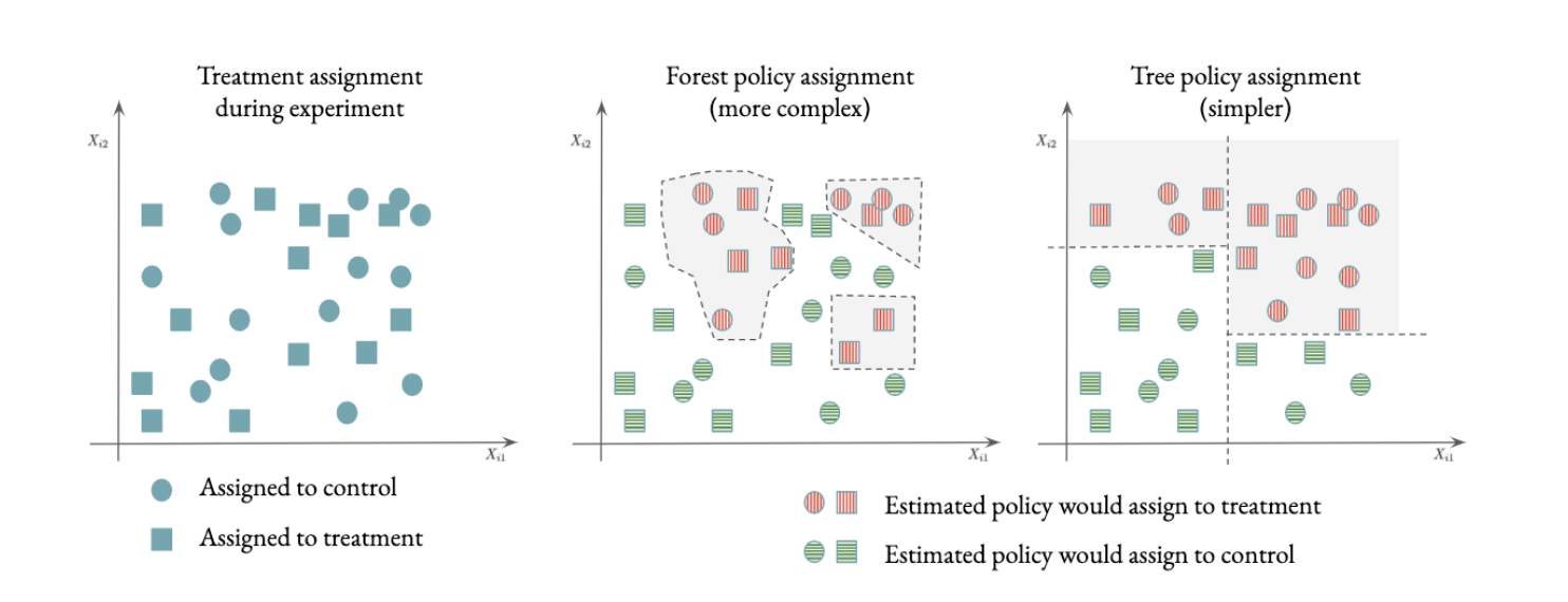
Figure 8.1: Optimal assignment according to different policies.
As outlined above, there are a variety of reasons that a policy maker may wish to restrict the treatment assignment policy. One disadvantage of using a flexible method (like causal forests) is that it can be difficult to explain eligibility criteria. As a result, similar individuals may have different treatment assignments, as illustrated in Figure 8.1. Athey & Wager (2020) developed an efficient method for estimating optimal policies with constraints on complexity, for example, if the policy is restricted to take the form of a tree, the resulting partition of the covariate space can be much simpler, as shown on the third panel of Figure 8.1, making it particularly easy to convey the eligibility criterion. The R software package policytree implements tree-based policies based on the methods described in Athey & Wager (2020), Zhou et al. (2018), and Sverdrup et al. (2020).
Once a treatment assignment policy has been estimated, we can evaluate its value. Specifically, we can estimate the counterfactual average outcome we would have observed if the treatment had been assigned according to the estimated policy. We can also compare it relative to an alternative, such as randomly assigning the treatment, or assigning everyone to the control condition. But an important caveat is that, just like with the predictive models we saw before, we cannot use the same data to estimate a policy and evaluate it, since that would lead to a biased estimate. Therefore, we usually need some form of sample splitting in which we estimate a policy using some portion of the data and then use the remaining portion to evaluate the performance of this policy. Forest-based methods are particularly convenient because each tree is fitted using only a subset of the data, so we can evaluate the value of assigning a particular observation to treatment or control where the assignment was determined using only the subset of trees that have never seen that observation. This means that forests have a built-in sample-splitting mechanism.
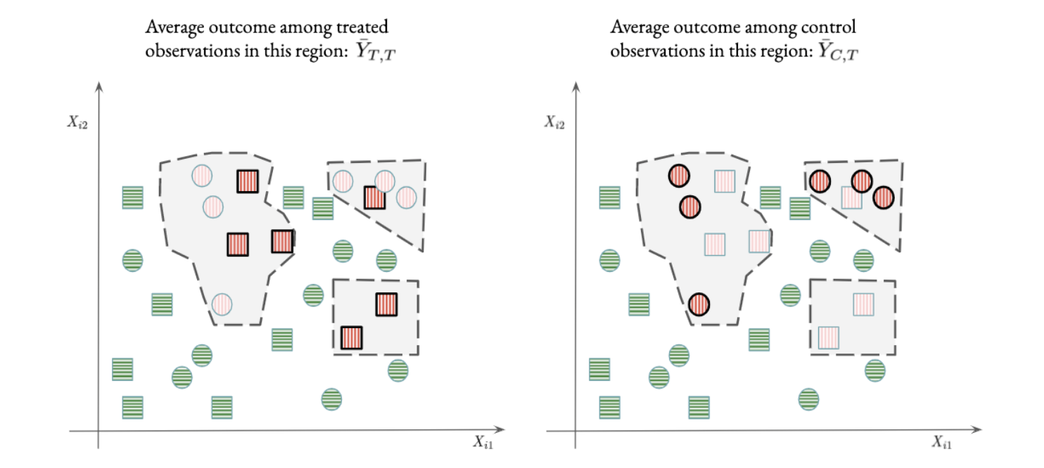
Figure 8.2: Evaluating a forest policy.
As an example, let’s say we would like to compare the forest policy displayed in Figure 8.1 to a baseline policy that assigns everyone to control. We begin by noting that the forest policy splits the observations into two groups: those that the forest policy would not treat (green colored, white background), and those that it would treat (red-colored, gray background). For the former group, both the forest policy and the baseline policies agree (neither treats), so the difference in expected outcomes for the two policies is exactly zero. For the latter group, we can estimate the value of treatment by computing the average outcome among those observations \(\bar{Y}_{T,T}\) (Figure 8.2, left panel, highlighted red squares), and subtract from that the average outcome among control observations in the group \(\bar{Y}_{C,T}\) (Figure 8.2, right panel, highlighted red circles). The final estimate equals this difference multiplied by the relative size of the treatment region (i.e., the fraction of observations inside the gray region), or 12/28=3/7 in the illustration, yielding \(3/7 (\bar{Y}_{T,T} - \bar{Y}_{C,T})\) .
Athey & Imbens (2016), Nie & Wager (2017), and Künzel et al. (2019) discuss issues that arise in constructing objective functions for heterogeneous treatment effect estimation.↩︎