11 Behavioral case study #2: Reducing vehicle booting among New York City drivers

In Section 1, we discussed some of our work in collaboration with the New York City Dept. of Finance (DOF) to encourage drivers to resolve their parking fines. We mentioned that our team initially developed nine new prototype emails to send to drivers warning them about their boot eligibility status. In this section, we will further discuss how we selected among these prototypes via experiments.

Rather than running a single trial testing ten treatment arms (the nine prototypes plus one control), we used a two-phase experimental design. The purpose of the first-stage design was to reveal a set of good arms for further testing during the second phase. The reason for this split into two phases was that running a single randomized controlled trial with ten treatment arms (nine prototypes and control) would be very expensive as well as potentially wasteful. A design that has the power to test hypotheses about each of the nine treatment arms against the control needs to be large enough that the payoff for each arm can be precisely estimated. Further, such an experiment is likely wasteful, since some arms may perform badly enough that precise estimates are not useful to policy makers, while other arms may be substantially similar, making it irrelevant which is chosen. In order to avoid this type of expense and waste, a pilot study can be used to narrow down the set of arms to be used in the primary experiment.

We conducted the first phase on the Amazon Mechanical Turk online platform. Participants were recruited and instructed to engage with a simulated email inbox. We asked them if they would rate the proposed subject lines as high-priority, and observed if they understood where to click in the email in order to resolve their parking fines. We collected about 1600 observations in three waves. In the first wave, for about 450 observations, we allocated arms with equal probability; then, in the second wave, for about 850 observations, we collected data using a linear Thompson sampling design; finally, the remaining observations were allocated to the control group. The adaptive data-collection wave ensured that many observations received the best treatments, while the last wave ensured that we had enough information about the control.

The next figure shows the evolution of non-contextual posterior probabilities over the course of the MTurk experiment, assuming a Beta-Bernoulli model (note: although the data-collection mechanism used information about contexts, we did not find any meaningful heterogeneity, so the non-contextual probabilities provide an approximation for the contextual probabilities that is easier to visualize and interpret).

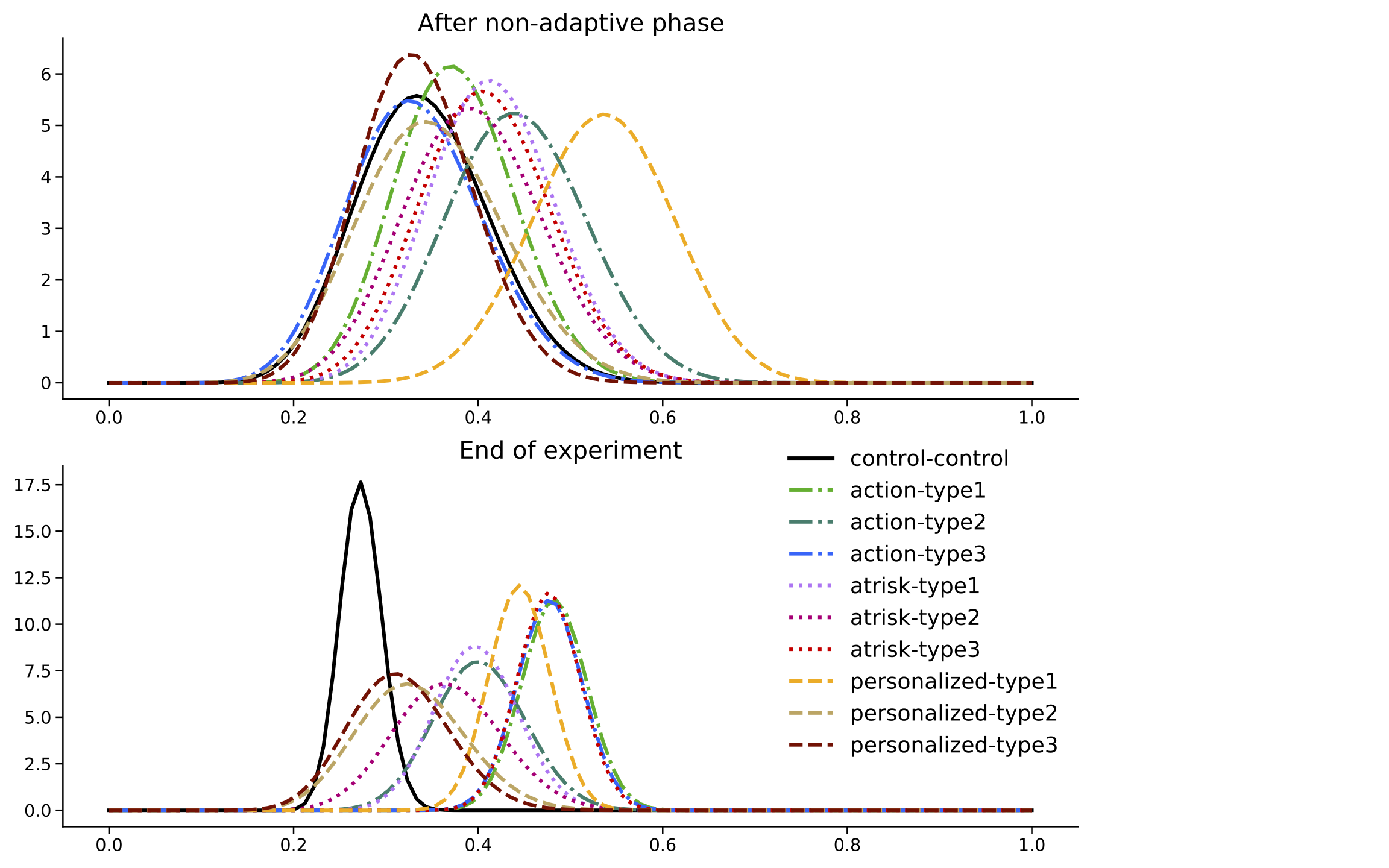
Figure 11.1: Evolution of (non-contextual) probabilities during the MTurk pilot. At the end of the experiment, results suggest that the control (black) has a lower average than most arms.

The experiment revealed two takeaways. First, at the end of the experiment the posterior distribution for the control arm (in black) was left-shifted compared to some of the new prototypes, suggesting that the performance of the control arm was inferior to them. Second, the prototypes named “action-type1” (light green), “action-type3” (blue) and “atrisk-type2” (red) had the largest posterior mean.

These results would suggest that, at the end of the experiment, some subset of the dominating arms could have been selected for further testing during the main experiment, since they had the highest posterior probabilities of being the best arm. However, due to implementation and legal constraints not anticipated when designing the pilot, these arms were not able to be implemented for further experimentation. In the end, the main experiment was run using two non-contextual variations that were very closely related to some of the best-performing arms.

The second and final phase of the experiment was a traditional randomized control trial that tested the effect of three arms (the two new prototypes and the control) on actual drivers in New York City. As we described in Section 1, our results suggested that our prototypes improved upon the control by increasing the engagement probability by around 8-10%.

Benefits of adaptive data collection

This case study demonstrates how a pilot study can be used to inform important details of the main experiment. However, the connection between pilot study and main experiment were imperfect, as technical and legal constraints meant that the select pilot arms could not be implemented exactly as in the pilot. In addition, a single experiment would have provided only limited validation of the general method.

Therefore, in order to illustrate the potential benefits of running an adaptive pilot experiment to select a small set of arms for further testing, let’s run a brief simulation exercise. In particular, we’ll show that by collecting data adaptively during the pilot we increase our chances of selecting good arms, which in turn increases the average value of the reward we attain at the selected arm.

We’ll consider a slightly simplified setting with ten arms, no contexts and a binary variable, but similar to the MTurk experiment in terms of effects and uncertainty: at each simulation, we draw a vector of true average arm values drawn from the Beta distribution such that they have mean 0.45 and standard deviation of 0.05. We will collect 1630 data points and decide which arms to submit for further testing. For simplicity, we also assume that in the second phase we can always discern which arm is best, so that all we need to ensure is that the best arm is within the set arms selected at the end of the first stage.

We consider three strategies for treatment assignment:

• Assign treatments uniformly at random, without any adaptivity, as in an RCT.
• Assign treatments uniformly at random for the first third of the experiment, then use a non-contextual Thompson sampling algorithm for the rest of the experiment.
• Assign treatments uniformly at random for the first third of the experiment, then use exploration sampling (Kasy & Sautmann (2019)) for the rest of the experiment.

Once the data is collected, we select the two arms with highest posterior probability of being the best arm according to a Bayesian model with a Beta(1, 1) prior and Bernoulli likelihood. The next figures show the results of 10,000 simulations.

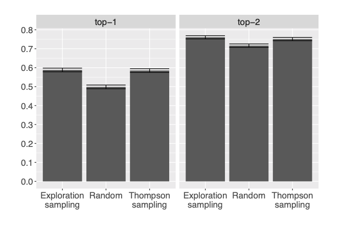
Figure 11.2: Comparison between different data collection strategies based on how often the true best arm had the highest posterior probability of being best (left) or was one of the two arms with highest posterior probability of being best (right). Error bars correspond to intervals defined by the mean probability, plus or minus 1.96 times the standard error of the relevant probabilities across 10,000 simulation runs.

Interestingly, we see that both Thompson sampling and exploration sampling select the correct arm roughly at the same rate, even though Thompson sampling is optimizing a different objective – minimizing mistakes during the experiment, as opposed to after it. This suggests that, although exploration sampling would have been more appropriate for our objective during the MTurk experiment, we would have likely obtained similar results. The next figure shows the benefit of adaptive experimentation in terms of the value of the arm that is eventually selected.

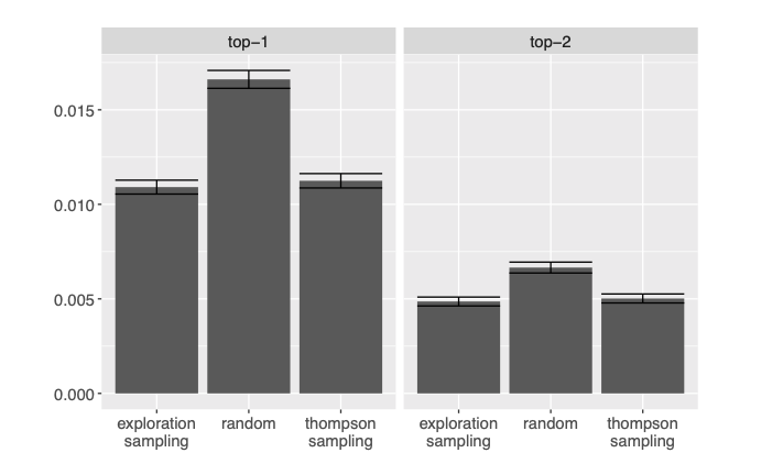
Figure 11.3: Comparison between different data collection strategies based on the difference in value between the true best and the arm that was eventually selected (so a smaller difference is better). Error bars correspond to intervals defined by the mean value, plus or minus 1.96 times the standard error of the relevant values across 10,000 simulation runs.

We see that although the three data-collection strategies are making a considerable number of mistakes, the figure above reveals that the difference in value between them is rather small in terms of expected value of the selected arms – although this can be relative: after all, a small change in the proportion of resolved parking fines can mean a large amount of money in the long run. In any case, this magnitude can be explained as follows. If the true difference between two arms is large, it is easier for us to tell them apart after collecting a small amount of data. If their differences are instead very small, we might not be able to distinguish between two arms, but we receive only a small penalty for picking the wrong one. Therefore it is in the cases of moderate differences that the algorithms mistakes tend to matter most. But it is precisely this case that reflects real-life situations most accurately, since in reality the experiment designer often chooses arms that are somewhat distinct from each other - and therefore have different effects - but they are still similar enough that a pilot study is necessary to decide between them.

Although the setting here was somewhat stylized, these results suggest that by employing adaptive experimental designs in the pilot experiment, we can increase our chances of including the best arm among the selected arms, and therefore also the value of the arm that was finally selected.