Tutorial: Post-Estimations
Author: Tianyu Du (tianyudu@stanford.edu)
This tutorial covers the toolkit in torch-choice for visualizing and analyzing models after model estimation.
Note: models demonstrated in this tutorial are for demonstration purpose only, hence we don't estimate them in this tutorial. Instead, this tutorial focuses on APIs to visualize and analyze models.
# import required dependencies.
from time import time

import numpy as np
import pandas as pd
import seaborn as sns
import matplotlib.pyplot as plt
import torch
import torch.nn.functional as F

from torch_choice.data import ChoiceDataset, JointDataset, utils
from torch_choice.model import ConditionalLogitModel, NestedLogitModel
from torch_choice.utils.run_helper import run
# let's get a helper
def print_dict_shape(d):
    for key, val in d.items():
        if torch.is_tensor(val):
            print(f'dict.{key}.shape={val.shape}')
Creating ChoiceDataset Object
We first create a dummy ChoiceDataset object, please refer to the data management tutorial for more details.
# Feel free to modify it as you want.
num_users = 100
num_items = 25
num_sessions = 500

length_of_dataset = 10000
# create observables/features, the number of parameters are arbitrarily chosen.
# generate 128 features for each user, e.g., race, gender.
user_obs = torch.randn(num_users, 128)
# generate 64 features for each user, e.g., quality.
item_obs = torch.randn(num_items, 64)
# generate 10 features for each session, e.g., weekday indicator.
session_obs = torch.randn(num_sessions, 10)
# generate 12 features for each session user pair, e.g., the budget of that user at the shopping day.
itemsession_obs = torch.randn(num_sessions, num_items, 12)
item_index = torch.LongTensor(np.random.choice(num_items, size=length_of_dataset))
user_index = torch.LongTensor(np.random.choice(num_users, size=length_of_dataset))
session_index = torch.LongTensor(np.random.choice(num_sessions, size=length_of_dataset))
# assume all items are available in all sessions.
item_availability = torch.ones(num_sessions, num_items).bool()

# initialize a ChoiceDataset object.
dataset = ChoiceDataset(
    # pre-specified keywords of __init__
    item_index=item_index,  # required.
    # optional:
    num_users=num_users,
    num_items=num_items,
    user_index=user_index,
    session_index=session_index,
    item_availability=item_availability,
    # additional keywords of __init__
    user_obs=user_obs,
    item_obs=item_obs,
    session_obs=session_obs,
    itemsession_obs=itemsession_obs)
ChoiceDataset(label=[], item_index=[10000], user_index=[10000], session_index=[10000], item_availability=[500, 25], user_obs=[100, 128], item_obs=[25, 64], session_obs=[500, 10], itemsession_obs=[500, 25, 12], device=cpu)
Conditional Logit Model
Suppose that we are creating a very complicated dummy model as the following. Please note that model and dataset here are for demonstration purpose only, the model is unlikely to converge if one estimate it on this dataset.
model = ConditionalLogitModel(formula='(1|constant) + (1|item) + (1|user) + (user_obs|item) + (item_obs|constant) + (session_obs|user) + (itemsession_obs|item) + (itemsession_obs|user)',
                              dataset=dataset,
                              num_users=num_users,
                              num_items=num_items)

# estimate the model... omitted in this tutorial.
ConditionalLogitModel(
  (coef_dict): ModuleDict(
    (intercept[constant]): Coefficient(variation=constant, num_items=25, num_users=100, num_params=1, 1 trainable parameters in total, device=cpu).
    (intercept[item]): Coefficient(variation=item, num_items=25, num_users=100, num_params=1, 24 trainable parameters in total, device=cpu).
    (intercept[user]): Coefficient(variation=user, num_items=25, num_users=100, num_params=1, 100 trainable parameters in total, device=cpu).
    (user_obs[item]): Coefficient(variation=item, num_items=25, num_users=100, num_params=128, 3072 trainable parameters in total, device=cpu).
    (item_obs[constant]): Coefficient(variation=constant, num_items=25, num_users=100, num_params=64, 64 trainable parameters in total, device=cpu).
    (session_obs[user]): Coefficient(variation=user, num_items=25, num_users=100, num_params=10, 1000 trainable parameters in total, device=cpu).
    (itemsession_obs[item]): Coefficient(variation=item, num_items=25, num_users=100, num_params=12, 288 trainable parameters in total, device=cpu).
    (itemsession_obs[user]): Coefficient(variation=user, num_items=25, num_users=100, num_params=12, 1200 trainable parameters in total, device=cpu).
  )
)
Conditional logistic discrete choice model, expects input features:

X[intercept[constant]] with 1 parameters, with constant level variation.
X[intercept[item]] with 1 parameters, with item level variation.
X[intercept[user]] with 1 parameters, with user level variation.
X[user_obs[item]] with 128 parameters, with item level variation.
X[item_obs[constant]] with 64 parameters, with constant level variation.
X[session_obs[user]] with 10 parameters, with user level variation.
X[itemsession_obs[item]] with 12 parameters, with item level variation.
X[itemsession_obs[user]] with 12 parameters, with user level variation.
device=cpu
Retrieving Model Parameters with the get_coefficient() method.
In the model representation above, we can see that the model has coefficients from intercept[constant] to itemsession_obs.
The get_coefficient() method allows users to retrieve the coefficient values from the model using the general syntax model.get_coefficient(COEFFICIENT_NAME).
For example, model.get_coefficient('intercept[constant]') will return the value of \(\alpha\), which is a scalar.
tensor([0.3743])
model.get_coefficient('intercept[user]') returns the array of \(\gamma_u\)'s, which is a 1D array of length num_users.
torch.Size([100, 1])
model.get_coefficient('session_obs[user]') returns the corresponding coefficient \(\theta_u\), which is a 2D array of shape (num_users, num_session_features). Each row of the returned tensor corresponds to the coefficient vector of a user.
torch.Size([100, 10])
Lastly, the itemsession_obs (a 12-dimensional feature vector for each \((i, s)\) pairs) affects the utility through both \(\kappa_i\) and \(\iota_u\). For each item (except for the first item indexed with 0, all coefficients of it are 0), the get_coefficient() method returns a 2D array of shape (num_items-1, num_itemsession_features).
The first row of the returned tensor corresponds to the coefficient vector of the second item, and so on.
model.get_coefficient('itemsession_obs[user]') provides the user-specific relationship between utility and item-session observables, \(\iota_u\), which is a 2D array of shape (num_users, num_itemsession_features). Each row of the returned tensor corresponds to the coefficient vector of a user.
torch.Size([24, 12])
torch.Size([100, 12])
Visualizing Model Parameters
Researchers can use any plotting library to visualize the model parameters. Here we use matplotlib to demonstrate how to visualize the model parameters.
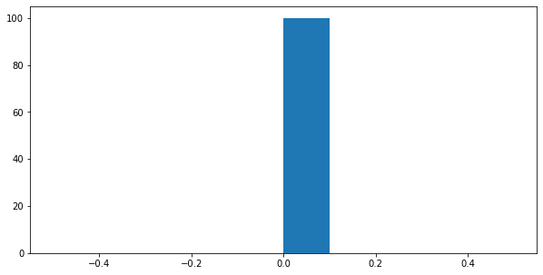
For example, we can plot the distribution of user fixed effect \(\gamma_u\)'s as the following.
- Researcher can use the
get_coefficient()method to retrieve the coefficient values.
- After estimating the model with GPU, the coefficient values are stored in the GPU memory. We need move the coefficient values to CPU memory and convert it to a numpy array before plotting.
- The tensor of individual fixed effects has shape (num_users, 1), you can use
squeeze()to remove the dimension of size 1. Since we haven't updated the model in this tutorial, the coefficient values are all zeros.
array([0., 0., 0., 0., 0., 0., 0., 0., 0., 0., 0., 0., 0., 0., 0., 0., 0.,
       0., 0., 0., 0., 0., 0., 0., 0., 0., 0., 0., 0., 0., 0., 0., 0., 0.,
       0., 0., 0., 0., 0., 0., 0., 0., 0., 0., 0., 0., 0., 0., 0., 0., 0.,
       0., 0., 0., 0., 0., 0., 0., 0., 0., 0., 0., 0., 0., 0., 0., 0., 0.,
       0., 0., 0., 0., 0., 0., 0., 0., 0., 0., 0., 0., 0., 0., 0., 0., 0.,
       0., 0., 0., 0., 0., 0., 0., 0., 0., 0., 0., 0., 0., 0., 0.],
      dtype=float32)
- Researcher can use
matplotlibto plot the distribution of the coefficient values. For example, the distribution plot of coefficients is helpful to identify potential groups of users with different preferences.
Nested Logit Model
The nested logit model has a very similar interface for coefficient extraction to the conditional logit model demonstrated above.
Consider a nested logit model with the same item-level model but with nest-level model incorporating user-fixed effect, category-fixed effect (specified by (1|item) in the nest_formula), and user-specific coefficient on a 64-dimensional nest-specific observable (specified by (item_obs|user) in the nest_formula).
The only difference is researcher would need to retrieve the coefficients of the nested logit model using the get_coefficient() method with the level argument.
NestedLogitModel.get_coefficient() Method.
nest_to_item = {
    0: [0, 1, 2, 3, 4],
    1: [5, 6, 7, 8, 9],
    2: [10, 11, 12, 13, 14],
    3: [15, 16, 17, 18, 19],
    4: [20, 21, 22, 23, 24]
}

nest_dataset = ChoiceDataset(item_index=item_index, user_index=user_index, num_items=len(nest_to_item), num_users=num_users, item_obs=torch.randn(len(nest_to_item), 64))
joint_dataset = JointDataset(nest=nest_dataset, item=dataset)
joint_dataset
No `session_index` is provided, assume each choice instance is in its own session.


JointDataset with 2 sub-datasets: (
    nest: ChoiceDataset(label=[], item_index=[10000], user_index=[10000], session_index=[10000], item_availability=[], item_obs=[5, 64], device=cpu)
    item: ChoiceDataset(label=[], item_index=[10000], user_index=[10000], session_index=[10000], item_availability=[500, 25], user_obs=[100, 128], item_obs=[25, 64], session_obs=[500, 10], itemsession_obs=[500, 25, 12], device=cpu)
)
nested_model = NestedLogitModel(nest_to_item=nest_to_item,
                                nest_formula='(1|user) + (1|item) + (item_obs|user)',
                                item_formula='(1|constant) + (1|item) + (1|user) + (user_obs|item) + (item_obs|constant) + (session_obs|user) + (itemsession_obs|item) + (itemsession_obs|user)',
                                num_users=num_users,
                                dataset=joint_dataset,
                                shared_lambda=False)
nested_model
NestedLogitModel(
  (nest_coef_dict): ModuleDict(
    (intercept[user]): Coefficient(variation=user, num_items=5, num_users=100, num_params=1, 100 trainable parameters in total, device=cpu).
    (intercept[item]): Coefficient(variation=item, num_items=5, num_users=100, num_params=1, 4 trainable parameters in total, device=cpu).
    (item_obs[user]): Coefficient(variation=user, num_items=5, num_users=100, num_params=64, 6400 trainable parameters in total, device=cpu).
  )
  (item_coef_dict): ModuleDict(
    (intercept[constant]): Coefficient(variation=constant, num_items=25, num_users=100, num_params=1, 1 trainable parameters in total, device=cpu).
    (intercept[item]): Coefficient(variation=item, num_items=25, num_users=100, num_params=1, 24 trainable parameters in total, device=cpu).
    (intercept[user]): Coefficient(variation=user, num_items=25, num_users=100, num_params=1, 100 trainable parameters in total, device=cpu).
    (user_obs[item]): Coefficient(variation=item, num_items=25, num_users=100, num_params=128, 3072 trainable parameters in total, device=cpu).
    (item_obs[constant]): Coefficient(variation=constant, num_items=25, num_users=100, num_params=64, 64 trainable parameters in total, device=cpu).
    (session_obs[user]): Coefficient(variation=user, num_items=25, num_users=100, num_params=10, 1000 trainable parameters in total, device=cpu).
    (itemsession_obs[item]): Coefficient(variation=item, num_items=25, num_users=100, num_params=12, 288 trainable parameters in total, device=cpu).
    (itemsession_obs[user]): Coefficient(variation=user, num_items=25, num_users=100, num_params=12, 1200 trainable parameters in total, device=cpu).
  )
)
For example, you can use the following code snippet to retrieve the coefficient of the user-fixed effect in the nest level model, which is a vector with num_users elements.
torch.Size([100, 1])
Similarly, by changing to level='item', the researcher can obtain the coefficient of user-specific fixed effect in the item level model, which is also a vector with num_users elements.
torch.Size([100, 1])
This API generalizes to all other coefficients listed above such as itemsession_obs[item] and itemsession_obs[user].
One exception is the coefficients for inclusive values, (often denoted as \(\lambda\)). Researchers can retrieve the coefficient of the inclusive value by using get_coefficient('lambda') without specifying the level argument (get_coefficient will disregard any level argument if the coefficient name is lambda). The returned value is a scalar if shared_lambda is True, and a 1D array of length num_nests if shared_lambda is False. In our case, the returned value is an array of length five (we have five nests in this model).
tensor([0.5000, 0.5000, 0.5000, 0.5000, 0.5000])